
Queuing theory and operations research is a huge subject that applies to an enormous range of situations. Queues are everywhere. At b-agile our core interest is identifying and optimising the queues in business processes: product, platform and service development, business operations, and digital, AI and organisational change.
What is queuing theory?
Queuing theory is the mathematical study of how waiting lines, or queues, form, function and become congested. It is also written as queueing theory, and called queue theory or waiting line theory.
At its core, a queuing situation has two parts:
- Someone or something that requests a service, usually called the customer, job or request.
- Someone or something that completes or delivers the service, usually called the server.
Two examples. At a bank, the customers are the people wanting to deposit or withdraw money and the servers are the tellers. For a printer, the customers are the print requests and the server is the printer.
Queuing theory looks at the whole system of waiting in line: the customer arrival rate, the number of servers, the number of customers, the capacity of the waiting area, the average time to complete a service, and the queuing discipline.
The queuing discipline is the rules of the queue: first in first out, last in first out, prioritised, or served in random order.
How did queuing theory start?
Queuing theory was introduced in the early twentieth century by the Danish mathematician and engineer Agner Krarup Erlang.
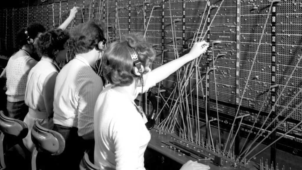
Erlang worked for the Copenhagen Telephone Exchange and wanted to analyse and optimise its operations. He set out to determine how many circuits were needed to give an acceptable level of service, so that people were not on hold, in a telephone queue, for too long. He also wanted to know how many operators were needed to handle a given volume of calls.
His analysis culminated in the 1920 paper "Telephone Waiting Times", which contained some of the first queuing models and became the foundation of applied queuing theory. The international unit of telephone traffic is called the erlang in his honour.
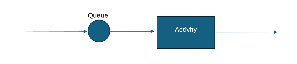
In queuing theory, every system can be simplified to entities queuing for activities. Call this sub-system managing customers queuing for service. To analyse it we need to know about:
The arrival process:
- How customers arrive, individually or in groups.
- The probability distribution of the time between arrivals, the inter-arrival time distribution.
- Whether the customer population is finite or infinite.
The service mechanism:
- The resources needed to start the service.
- How long the service takes, the service time distribution.
- How many servers there are.
- How the servers are arranged: in series with separate queues, or in parallel with one queue for all.
- The pre-emption policy: whether a server can interrupt a customer for an emergency.
The queue's characteristics:
- How the next customer is chosen: first in first out, first come first served, last in first out, or at random. This is the queue discipline.
- Whether there is balking (customers avoid joining a long queue), reneging (customers leave if they wait too long) or jockeying (customers switch queues for faster service).
- Whether the queue's capacity is finite or infinite.
Queuing theory uses Kendall notation to classify the types of queuing system, or nodes. A node is written A/S/c/K/N/D, where:
- A is the arrival process.
- S is the mathematical distribution of the service time.
- c is the number of servers.
- K is the capacity of the queue, omitted if unlimited.
- N is the number of possible customers, omitted if unlimited.
- D is the queuing discipline, assumed first in first out if omitted.
Think of a cash machine. It serves one customer at a time, first in first out, with randomly distributed arrivals and service times, unlimited queue capacity and an unlimited number of possible customers. Queuing theory describes it as an M/M/1 queue, where M stands for Markovian, a statistical process for describing randomness.
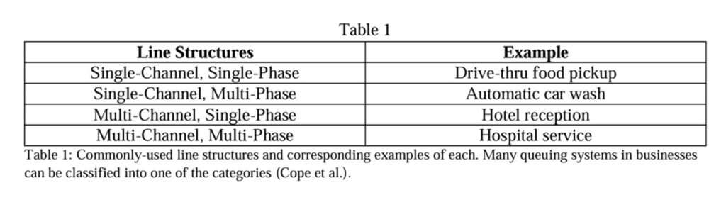
Most queuing systems in business fall into one of these line forms:
Why does queuing theory matter?
Waiting in line is part of everyday life because, as a process, it serves several important functions. Queues are a fair and essential way of handling the flow of customers when resources are limited. Without a queue process, overcapacity produces bad outcomes.
When too many visitors arrive at a website, it slows and crashes unless it can change the rate at which it processes requests or queue the visitors. Imagine planes waiting for a runway. With too many planes and no queue, all of them trying to land at once would have real safety implications.
Queuing theory matters because it describes the features of a queue, such as the average wait time, and provides the tools to optimise it. For a business, queuing theory in operations research informs the design of efficient, cost-effective workflow systems.
Queuing situations involve uncertainty in inter-arrival and service times, so analysing them takes probability and statistics.
The performance metrics we focus on are:
- The expected wait before service, and before completion.
- The probability of waiting longer than a given interval.
- The average queue length.
- The probability of the queue exceeding a given length.
- The expected server utilisation and the periods of full occupation. Assigning a cost to customer wait time and to server idle time helps design a cost-effective system.
Teams need answers to a few key questions to evaluate alternatives and improve a situation:
- Is reducing the service time worth the effort?
- How many servers are needed?
- Should customers be prioritised?
- Is the waiting area adequate?
There are two main ways to answer them: analytic methods, which is queuing theory, and computer simulation.
Queuing theory works for simple systems. More complex systems are usually analysed with simulation, more precisely discrete-event simulation.
A simple simulation
Suppose customers arrive with inter-arrival times uniformly distributed between one and three minutes, so every value in that range is equally likely. Suppose service times are uniformly distributed between 0.5 and 2 minutes.
We have two independent distributions. We can generate lists of times by sampling from them in Excel: 1+(3-1)*RAND() for inter-arrival times and 0.5+(2-0.5)*RAND() for service times.
Suppose our two lists, rounded to one decimal place, are:
| Inter-arrival times | Service times |
|---|---|
| 1.9 | 1.7 |
| 1.3 | 1.8 |
| 1.1 | 1.5 |
| 1.0 | 0.9 |
| etc. | etc. |
Consider the system at time zero (T=0) with no customers. What happens next?
After 1.9 minutes a customer arrives and is served immediately, because the queue is empty and the server is idle.
At T=3.2, after 1.3 more minutes, another customer arrives and joins the queue because the server is busy.
At T=3.6, 1.7 minutes after service began, the first customer finishes and leaves. The next customer starts service, which will end at T=5.4 after 1.8 minutes.
Another customer arrives at T=4.3, 1.1 minutes after the previous arrival, and joins the queue.
At T=5.3, 1.0 minutes later, another arrives and joins the queue. Two customers are now waiting.
At T=5.4 the current customer finishes. The customer at the head of the queue begins service, which will end at T=6.9 after 1.5 minutes.
Obviously this is best done by a computer. Summarised as a list of events:
| Time T | What happened |
|---|---|
| 1.9 | Customer arrives, starts service scheduled to end at T=3.6 |
| 3.2 | Customer arrives, joins queue |
| 3.6 | Service ends. Customer at head of queue starts service, scheduled to end at T=5.4 |
| 4.3 | Customer arrives, joins queue |
| 5.3 | Customer arrives, joins queue |
| 5.4 | Service ends. Customer at head of queue starts service, scheduled to end at T=6.9 |
This is discrete-event simulation: we emulate the queuing system by focusing on specific events over time, the arrivals and service completions at T=1.9, 3.2, 3.6, 4.3, 5.3, 5.4 and so on.
From the simulation we can derive statistics about the system, such as the average time a customer spends queuing and being served. Two customers have completed the whole process. The first arrived at 1.9 and left at 3.6, spending 1.7 minutes in the system. The second arrived at 3.2 and left at 5.4, spending 2.2 minutes. The average time in the system is (1.7 + 2.2) / 2 = 1.95 minutes.
We can also calculate queue length statistics. The queue is 0 from T=0 to 3.2, 1 from 3.2 to 3.6, 0 from 3.6 to 4.3, 1 from 4.3 to 5.3, and 2 from 5.3 to 5.4. The time-weighted average queue size is:
[0(3.2−0) + 1(3.6−3.2) + 0(4.3−3.6) + 1(5.3−4.3) + 2(5.4−5.3)] / 5.4 = 0.296
Simulation was applied to management in the late 1950s for queuing and stock control problems. Monte Carlo simulation modelled warehouses, oil depots and queues such as supermarket checkouts. The name comes from the famous gambling city in Monaco, because the random numbers from a roulette wheel are much like the random numbers a computer generates in a simulation.
The benefits of simulation over queuing theory:
- It handles time-dependent behaviour more effectively.
- The mathematics of queuing theory is complex and only applies to certain statistical distributions. The mathematics of simulation is straightforward and works with any distribution.
- In some scenarios it is nearly impossible to construct the equations queuing theory needs, for example with queue switching or queue-dependent work rates.
- Simulation is far easier for managers to understand and use.
The drawback is that simulation makes it hard to find the optimal solution. Linear programming has algorithms that find the optimum automatically. Optimising a simulation is trial and error:
- Make a change.
- Run the simulation to see whether it improved things.
- Repeat as necessary.
Once we have a model we can use it to:
- Understand the current system. For example, identify the factors causing delays in factory production.
- Explore changes to improve it. Add machines, speed them up, or reduce idle time through better maintenance.
- Design a new system from scratch. For example, work out the resource levels and placement in an airport terminal that meet the statistical requirements at minimum cost.
Little's Law
Instead of building complex mathematical models with many variables, a business can use a simpler, more flexible model such as Little's Law.
It is written as L = λW, where L is the average number of items in a system, λ is the average arrival rate, and W is the average time an item waits. The average length of a queue in a steady state is the rate at which customers join it multiplied by the average time they spend in it.
Despite its apparent simplicity, Little's Law is powerful because the relationship does not depend on the distribution of arrivals or of service time. It holds for any service order or queuing principle.
Applying it gives you a simplified analysis of a complex system by looking only at queue length and wait time. That simplicity is also why it is not often used in formal queuing theory: the analysis may be too simple to represent a queuing model accurately. It still works well for overseeing ongoing operations. Each of the three averages it relates is a clear measure of how effective a process is, and any fault in the system shows up in at least one of them.
Little's Law connects the capacity of a queuing system, the average time spent in it and the average arrival rate without knowing anything else about the queue:

It can be rearranged to solve for either of the other two variables:


Where:
- L is the average number of customers in the system.
- λ (lambda) is the average arrival rate into the system.
- W is the average time spent in the system.
Lean and Kanban would not exist without Little's Law and its queuing models. For business applications it is usually written as:

Read more in Little's Law: understand your process.
A small number of references on queuing theory and operations research
Anderson, David R. et al. Quantitative Methods for Business. 12th ed. Mason, Ohio: South-Western, 2012.
Beasley, J. E. "OR-Notes." Brunel University London personal pages, 2005.
Byrd, Jack, Jr. "The Value of Queueing Theory." Interfaces 8.3 (1978): 22–26.
Cope, Robert F., III, Rachelle F. Cope and Harold E. Davis. "Disney's Virtual Queues: A Strategic…" Journal of Business & Economics Research 6.10 (2008): 13–20.
Cope, Rachelle F. et al. "Innovative Knowledge Management at Disney: Human Capital and Queuing Solutions for Services." Journal of Service Science 4.1 (2011): 13–20.
De Lange, Robert, Ilya Samoilovich and Bo van der Rhee. "Virtual Queuing at Airport Security Lanes." European Journal of Operational Research 225.1 (2013): 153–165.
Dickson, Duncan, Robert C. Ford and Bruce Laval. "Managing Real and Virtual Waits in Hospitality and Service Organizations." Cornell Hotel and Restaurant Administration Quarterly 46.1 (2005): 52–68.
Dudin, Alexander et al. "Multi-Server Queueing System with a Generalized Phase-Type Service Time Distribution as a Model of Call Center with a Call-Back Option." Annals of Operations Research 239.2 (2016): 401–428.
Katz, K., B. Larson and R. Larson. "Prescription for the Waiting in Line Blues." Sloan Management Review (Winter 1991): 44–53.
Kimes, Sheryl S. E. "The Role of Technology in Restaurant Revenue Management." Cornell Hospitality Quarterly 49.3 (2008): 297–309.
Little, John D. C. "Little's Law as Viewed on Its 50th Anniversary." Operations Research 59.3 (2011): 536–549.
Nelson, Emily. "The Art of Queueing up at Disneyland." Journal of Tourism History 8.1 (2016): 47–56.
Niles, Robert. "The Economics of How Disney Got from E Tickets to Paid Fastpasses." Theme Park Insider, 2018.
Simchi-Levi, David and Michael A. Trick. "Introduction to 'Little's Law as Viewed on Its 50th Anniversary.'" Operations Research 59.3 (2011): 535.
Taha, Hamdy A. "Queueing Theory in Practice." Interfaces 11.1 (1981): 43–49.