
Little’s Law – Understand your Process

As simple as Little’s Law is, its an incredibly powerful tool for understanding the performance of queues over time. Understanding the behaviour of processes is fundamental to running an effective efficient process.
Little’s Law explained
Little’s law is a theorem by John Little which states: the long-term average number L of customers in a stationary system is equal to the long-term average effective arrival rate λ multiplied by the average time W that a customer spends in the system.
In place of developing complex mathematical models with a number of variables to consider, businesses can use simpler, more flexible models such as Little’s law.
Little’s law is simply written as L=λW, where L represents the average number of items in a system, λ denotes the average arrival rate of items, and W indicates the average wait time of an item.
Little’s law states that the average length of a queue in steady state is given by the product of the rate at which customers enter the line and the average amount of time they spend in line.
Despite the perceived simplicity of the formula, Little’s law is powerful because the relationship is not dependent on the distribution of arriving customers or service time. Little’s law holds for any service order or queuing principle.
An application of Little’s law can provide a simplified analysis of complex systems by explicitly examining just queue length and wait time as opposed to considering a number of other factors. Despite the benefits of Little’s law, such a highly flexible model is not often used in queuing theory because the analysis is perhaps too simplified to provide an accurate representation of queuing models.
Little’s law may still function well in in overviewing ongoing operations. Although Little’s law relates three distinct average statistics, each value is a clear measure of the effectiveness of a process. Any fault in the system would likely be manifested in at least one of the averages.
Example notation:
- L is the long-term average number of customers in the system.
- λ is the long-term average effective arrival rate.
- W is the average time that a customer spends in the system.
- L = λ W is Little’s law.
This is often described as:
Work In Process (L) = Cycle Time (W) * Throughput (λ)
Throughput in the definition above λ is the long-term average effective departure rate. See assumptions below.
Little’s law assumptions:
- Conservation of flow, meaning the average arrival rate equals the average departure rate.
- All work that enters the system then flows through to completion.
- The total number of items is roughly the same at the beginning and at the end.
- The system is “stable”, meaning the average age of items are neither increasing or decreasing
- All measurement units are consistent.
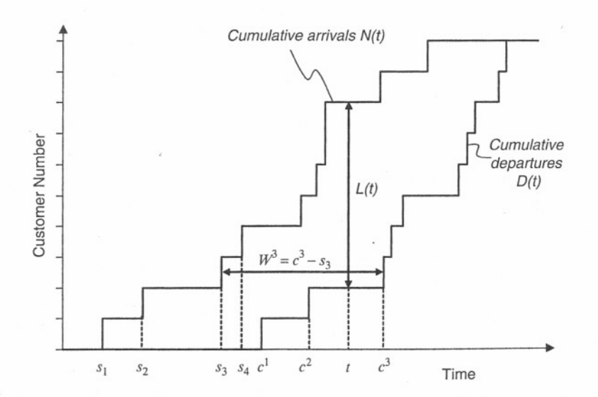
Cumulative arrivals/departures diagram by John Little
The Little’s Law calculation is indeed exact, but it is only exact in contexts when a specific set of assumptions are fulfilled. Those assumptions are for the time period under observation.
Think about the following situation. Which assumptions are being violated?

If we calculated two time periods we would see wildly different results, that tells us that the process is unstable and violates one or more of Little’s Law.
The net effect of violating Little’s assumptions is that you have destabilized your process–as evidenced by the equation not working. System stability is important because it is impossible to optimize a process that is inherently unstable.
Assumption 5 is pretty obvious. Use the same units. If Throughput is Days then we would use the same unit for Cycle Time
Assumptions 1 and 3 are equivalent. The assumptions refer to system stability but provide no guidance on the actual amount of Work in Process.
Assumption 2 is interesting but often ignored. In various kinds of work we perform we may abandon work occasionally. Although if we are abandoning a lot of work this may indicate process instability.
Assumption 4 is the most important assumption. What Little’s Law describes is the relationship of increasing the arrival rate increases Work in Process causing work in the system to age.
Queues are everywhere from ordering food at McDonalds, standing in a supermarket checkout queue, buying tickets to a popular gig, to various business and product development processes. Little Law’s applies to all types of queues.
For example, if you’re waiting in line at a Starbucks, Little’s Law can estimate how long it would take to get your coffee.
Assume there are 15 people in line, one server, and 2 people are served per minute. To estimate this, you’d use Little’s Law in the form:

Showing that you could expect to wait 7.5 minutes for your coffee.


So Little’s Law provides a simplified view of complex queuing systems and we can see the results of any changes in the queuing system in changes in the long term averages. Little’s Law however cannot help us understand what may need to change in the queue to optimise the flow of value.
For more on queuing theory check our blog here